Gradient checking
Back-propagation is a tricky algorithm and sometimes a bugged implementation of it might still seem to work properly but it would not ensure a good minimization.
In order to find out bugs in back-propagation a technique called gradient checking can be used.
Until now we more or less accepted that provided formulas would compute the derivative of the cost function and numerical gradient checking gives us a method to verify that your implementation actually computes the derivative of the cost function $J(\Theta)$.
Suppose that out cost function looks like this and that $\Theta \in \mathbb{R}$
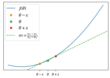
If we want to estimate the derivative we will take $\theta-\epsilon$ and $\theta+\epsilon$ where $\epsilon \approx 0$ and we will compute the slope of the line passing per $\theta-\epsilon, \theta+\epsilon$
\[\frac{d}{d\theta}\approx\frac{J(\theta+\epsilon)-J(\theta - \epsilon)}{2\epsilon}\]For $\epsilon$ small enough this numerical approximation becomes actually the derivative $\frac{d}{d\theta}$ but in order not to incurr in numerical problems we can use a $\epsilon \approx 10^{-4}$
In the case of $\theta \in \mathbb{R}^n$ we can use this strategy to check the gradient
\[\begin{align} & \frac{\partial}{\partial\theta_1}J(\theta) \approx \frac{J(\theta_1 + \epsilon,\theta_2,\dots,\theta_n) - J(\theta_1-\epsilon,\theta_2,\dots,\theta_n)}{2\epsilon}\\ & \frac{\partial}{\partial\theta_2}J(\theta) \approx \frac{J(\theta_1, \theta_2 + \epsilon,\dots,\theta_n) - J(\theta_1,\theta_2-\epsilon,\dots,\theta_n)}{2\epsilon}\\ & \;\; \vdots \\ & \frac{\partial}{\partial\theta_n}J(\theta) \approx \frac{J(\theta_1,\theta_2,\dots,\theta_n + \epsilon) - J(\theta_1,\theta_2,\dots,\theta_n-\epsilon)}{2\epsilon} \end{align}\]Random initialization
When performing optimization (e.g. gradient descent) we need to choose some initial value for $\Theta$ and it is possible to initialize $\Theta$ to a vector of $0$. While this strategy works when using logistic regression it doesn’t when training an ANN. Let’s take the example of a simple ANN where $\Theta_{ij}^{(l)}$ is set to $0$ for all $i, j, l$
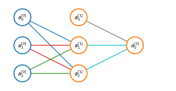
This will result in both of the hidden units $\color{blue}{a_1^{(2)}, a_2^{(2)}}$ will compute the same function of each input. This means that for every training example you will end up with $\color{blue}{a_1^{(2)} = a_2^{(2)}}$ and it can be shown also that $\color{blue}{\delta_1^{(2)} = \delta_2^{(2)}}$. Consequently
\[\color{blue}{\frac{\partial}{\partial\Theta_{01}^{(1)}}J(\Theta)=\frac{\partial}{\partial\Theta_{02}^{(1)}}J(\Theta)}\]and this means that even after one gredient descent update $\color{blue}{\Theta_{01}^{(1)}=\Theta_{02}^{(1)}}$. And the same goes for $\color{red}{\Theta_{01}^{(1)}=\Theta_{02}^{(1)}}$ and $\color{green}{\Theta_{01}^{(1)}=\Theta_{02}^{(1)}}$.
In order to get around this proble an ANN is randomly initialized. Each $\Theta_{ij}^{(l)}$ is initialized to a random value in $[-\epsilon, \epsilon]$
The random initialization of parameters $W^{[1]}$ (w1) can be done as:
constant = 0.01
w1 = np.random.rand(3,3) * constant
w1
array([[0.00353591, 0.00491842, 0.00794126],
       [0.00999681, 0.00271361, 0.00033436],
       [0.00869346, 0.00907858, 0.00824595]])
where constant is typically $0.01$, the reason being that if the wigths are too large, the activation function $a^{[1]}$ will output large values and gradient descent will be very slow.
When training shallow neural networks constant=0.01 is ok but when training deep neural networks you might want to chose different constant, but usually it wiil end up being a relatively small number.