Non-linear hypothesis with SVMs

In this section we will see how kernels enable SVMs to model complex non-linear data. Suppose we have a dataset like that in Figure 22.

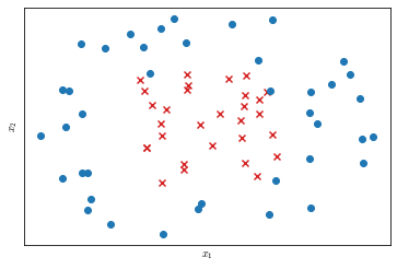
png — Figure 22. Non linear data scattered on its features space $(x_1, x_2)$. In this plots coordinates are randomly generated to fill two ellipses.

We could manually design an hypothesis with high order polynomial features to model the data, but is there a better way to choose the features?

Kernels

In this section we will start to explore the idea of kernels to define new features.

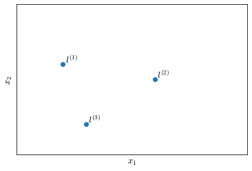
Let’s manually choose three points in the feature space $(x_1, x_2)$, that we will call the landmarks $l^{(1)}, l^{(2)}, l^{(3)}$ (Figure 23). We are going to define our as a measure of similarity between the training examples and the landmarks.

png — Figure 23. Three landmarks points chosen manually

Given an example $x$, we will define three features $f_1, f_2, f_3$:

\[\begin{align} & f_1 = k(x, l^{(1)}) = \exp\left({-\frac{\| x - l^{(1)}\|^2}{2 \sigma^2}}\right) \\ & f_2 = k(x, l^{(2)}) = \exp\left({-\frac{\| x - l^{(2)}\|^2}{2 \sigma^2}}\right) \\ & f_3 = k(x, l^{(3)}) = \exp\left({-\frac{\| x - l^{(3)}\|^2}{2 \sigma^2}}\right) \end{align}\]

where $k$ stands for kernel and is a function that measure similarity and $| x - l^{(i)}|$ is the euclidean distance between the example $x$ and the landmark point $l^{(i)}$; $\sigma$ is called the bandwidth parameter and determines the steepness of the Gaussian distribution. In particular the specific kernel $k$ used here is called the Gaussian kernel.

Let’s explore more in detail the first landmark, whose numerator can be also written as the square of the component-wise distance of the vector $x$ from the vector $l^{(1)}$:

\[f_1=k\left( x, l^{(i)} \right) = \exp \left( -\frac{\left \| x - l^{(1)} \right \|^2}{2\sigma^2}\right) = \exp \left( -\frac{\sum_{j=1}^n \left(x_j-l_j^{(1)} \right)^2}{2\sigma^2} \right)\]

When $x \approx l^{(1)}$, the euclidean distance between $x$ and $l^{(1)}$ will be $\approx 0$ and $f_1 \approx 1$

\[f_1 \approx \exp \left ( - \frac{0^2}{2 \sigma^2} \right ) \approx 1\]

Conversely, when $x$ is far from $l^{(1)}$ the euclidean distance between $x$ and $l^{(1)}$ will be a large number and $f_1 \approx 0$

\[f_1 = \exp \left( - \frac{\text{large number}^2}{2 \sigma^2} \right) \approx 0\]

To summarize:

\[f_1 \approx \begin{cases} 1 & \text{if } x \approx l^{(1)} \\ 0 & \text{if } x \neq l^{(1)} \end{cases}\]

Since we have three landmark points $l^{(1)}, l^{(2)}, l^{(3)}$, given an example $x$ we can define three new features $f_1, f_2, f_3$.

Similarity function

Let’s take a look at the similarity function $k$. Suppose

\[l^{(1)} = \begin{bmatrix}3\\5\end{bmatrix}, \quad f_1 = \exp \left( -\frac{\left \| x - l^{(1)} \right \|^2}{2\sigma^2}\right)\]

By looking at Figure 24, we can see how $f_1 \to 1$ when $x_1 \to 3$ and $x_2 \to 5$, where $(3, 5)$ are the coordinates of $l^{(1)}$.

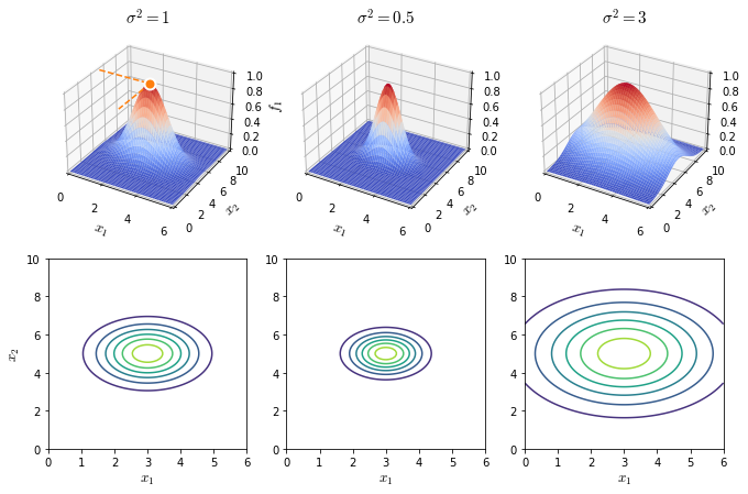
png — Figure 24. Three-dimensional surface and contour plot of the value the gaussian kernel $f_1$ as a function of the features $x_1$ and $x_2$. The three couple of plots are views of the kernel values when $\sigma^2= 1, 0.5, 3$ respectively.

It is also interesting to notice the effect of different values of $\sigma^2$ on $f_1$ output. When $\sigma^2$ decreases, $f_1$ falls to $0$ much more rapidly when $x$ stray from $l^{(1)}$. Conversely if the value of $\sigma^2$ is large the decay of $f_1$ is much slower.

Multiple landmarks

Let’s get back to Figure 23 and let’s try to put together what we have learned in the case of multiple landmarks.

We have three features $f_1, f_2, f_3$ and our hypothesis:

\[y = 1 \quad \text{if} \quad \theta_0 + \theta_1f_1 + \theta_2f_2 + \theta_3f_3 \geq 0\]

Suppose that we have run our learning algorithm and came up with the following parameters

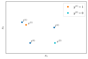
\[\theta= \begin{bmatrix} 0.5 \\ 1 \\ 1 \\ 0 \end{bmatrix}\]

Now let’s consider various training examples placed on the features space $(x_1, x_2)$ represented on Figure 25.

Training example $x^{(1)}$ is close to $l^{(1)}$, hence $f_1 \approx 1$ while $f_2, f_3 \approx 0$. Its prediction will be:

\[\begin{align} h_\theta(x^{(1)}) & = \theta_0 + \theta_1 \cdot 1 + \theta_2 \cdot 0 + \theta_3 \cdot 0 \\ &= -0.5 + 1 \\ &= 0.5 \geq 1 \\ & \to y^{(1)} = 1 \end{align}\]

Training example $x^{(2)}$ is far from any landmark, hence $f_1, f_2, f_3 \approx 0$ and $y^{(2)} \approx -0.5$

png — Figure 25. Manually placed landmarks as in Figure 23 and training example falling close or far from landmarks.

Choice of the landmarks

Until now we manually picked the landmarks, in an SVM landmarks are defined as exactly the same coordinates as the points in the training set. This means that when an input is fed to the trained algorithm, it calculates how close it is to points in the training set.

SVM with kernels

By defining the landmarks as the example coordinates means that if we have an $m \times n$ training set where each example $x^{(i)} \in \mathbb{R}^{n+1}$ space, we are going to define $m$ features (one for each training example), so that we will have our feature vector $f \in \mathbb{R}^{m+1}$ and also our parameter vector $\theta \in \mathbb{R}^{m+1}$.

The training for an SVM with kernels will be

\[\min_\theta C \sum^m_{i=1}y^{(i)} \text{cost}_1 \underbrace{\left(\theta^T f^{(i)}\right)}_{ \neq \theta^Tx^{(i)}} + \left( 1- y^{(i)}\right) \text{cost}_0 \left( \theta^T f^{(i)}\right) + \frac{1}{2} \sum^{\overbrace{n}^{m}}_{j=1}\theta^2_j\]

SVMs can also be used without kernels, and they are usually referred to as SVMs with linear kernels; it means that they will predict $y=1 \to \theta^Tx \geq 0$. This is usually the case when the number of features $n$ is large and the number of examples $m$ is small and you want to model the hypothesis as a linear function in order to prevent overfitting.

SVM hyper-parameters

When training an SVM, regardless of what kernel you use you will have to set the parameter $C$. Additionally, when using a Gaussian kernel, you will need to set the parameter $\sigma^2$. Both these hyper-parameters affect the bias vs variance trade-off

misclassification penalty $C \approx \frac{1}{\lambda}$:
- large $C$: Lower bias, higher variance
- small $C$: Higher bias, lower variance
bandwidth parameter $\sigma^2$, as we can infer from the figure with the gaussian and contour plots:
- Large $\sigma^2$: features $f_i$ vary more smoothly; higher bias, lower variance
- Small $\sigma^2$: features $f_i$ vary more abruptly; lower bias, higher variance

Implementation details

SVM optimization

In optimization implementations, usually the term $\sum^{\overbrace{n}^{m}}_{j=1}\theta^2_j$ is calculated as $\theta^T\theta$.

When optimizing an SVM algorithm, since $\theta \in \mathbb{R}^{m+1}$, we could end up with a huge number of parameters and $\theta^T\theta$ becomes inefficient or computationally impossible.

For this reason the term is usually slightly changed to $\theta^TM\theta$, where $M$ is a matrix that makes the computation much easier.

Incidentally, this implementation trick is also what prevents the kernel strategy to be applied to other learning algorithms. Kernels can be used with logistic regression too, however the $\theta^TM\theta$ would not be as useful as with SVMs, and consequently computation would not scale with the number of examples.

Other kernel tricks

Many numerical tricks are used in the implementations of SVMs and, while most of the times SVMs are used with linear of Gaussian kernels, they can accept other similarity functions. However not any function will work with SVMs and, in order to prevent divergence during training (due to the cited numerical tricks), they need to satisfy a technical condition called Mercer’s Theorem.

Feature scaling with Gaussian kernel

If using a Gaussian kernel and if features have very different scales you do need to perform feature scaling.

Logistic regression vs SVMs

In principle, to choose when to use logistic regression instead of SVMs, depends on the shape of your training set $(m, n)$, where $n$ is the number of features and $m$ is the number of training examples.

If $n$ is large relatively to $m$ ($\geq 1$ orders of magnitude): use logistic regression or SVM with linear kernel.

If $n$ is small ($n \in [1, 1000]$) and $m$ neither small nor big ($m \in [10, 10000]$): use SVM with Gaussian kernel.

If $m$ is large relatively to $n$: create or add more features and use logistic regression or SVM with linear kernel.

We couple logistic regression with SVM with linear kernel because they tend to have very similar performance. It is important to notice that in all these regimes neural networks are likely to work well but may be slower to train.