Regularization
When your model is overfitting your data (high variance) you can either get more data, which may not always be possible, or apply regularization.
We already talked about regularization in ML8, where the cost function of logistic regression is regularized and the regularization is mediated by the regularization parameter $\lambda$
\[\begin{equation} J(w,b)=\frac{1}{m}\sum_{i=1}^m\mathcal{L}\left(\hat{y}^{(i)},y^{(i)}\right)+\frac{\lambda}{2m}\|w\|_2^2 \end{equation} \label{eq:l2reg} \tag{1}\]where $|w|_2^2$ is called the $L_2$ norm of the vector $w$ and consequently $\eqref{eq:l2reg}$ is called $L_2$ regularization.
\[\|w\|_2^2 =\sum^{n_x}_{j=1}w_j^2=w^Tw\]$L_2$ is the most common type of regularization however sometimes $L_1$ regularization is used with
\[\frac{\lambda}{2m}\|w\|_1 = \frac{\lambda}{2m}\sum_{i=1}^{n_x}|w|\]This will cause $w$ to be sparse (have many zeros) and sometimes this can help compressing the model because the representation of zeros might sometimes require less memory than a non-zero number. However, this has a relatively small effect and usually $L_2$ regularization is preferred in deep-learning problems.
Regularized cost function in a neural network
In a neural network out cost function is a function of parameters in all $L$ layers and consequently its regularization sums over all the parameter matrices $w^{[l]}$ of each layer $l$:
\[\begin{equation} J(w^{[1]},b^{[1]}, \dots, w^{[L]},b^{[L]})=\frac{1}{m}\sum_{i=1}^m\mathcal{L}\left(\hat{y}^{(i)},y^{(i)}\right) + \underbrace{\frac{\lambda}{2m} \sum_{l=1}^L \|w^{[l]}\|^2}_\text{regularization} \end{equation} \label{eq:l2regnn} \tag{2}\]where the norm $| w^{[l]} |^2$ is
\[\| w^{[l]} \|^2=\sum_{i=1}^{n^{[l-1]}}\sum_{j=1}^{n^{[l]}}(w^{[l]}_{ij})^2 \qquad w \in R^{n^{[l-1]}\times n^{[l]}}\]This norm is called the Frobenius norm of a matrix and is denoted with $| w^{[l]} |_F$
Regularized backpropagation
When backpropagating error across the neural network (before regularization) you obtain $dw^{[l]}$ at each level $l$ and then update $w^{[l]}$
\[\begin{aligned} dW^{[l]} & = \overbrace{\frac{1}{m} dZ^{[l]} A^{[l-1]T}}^\text{from backpropagation} = dW^{[l]}_{bp} \\ w^{[l]} :& = w^{[l]}-\alpha \cdot dw^{[l]} \end{aligned} \qquad \qquad \qquad dW^{[l]} = \frac{\partial J}{\partial w^{[l]}}\]When the regularization term is added to the objective function $\eqref{eq:l2regnn}$ you obtain from backpropagation $dW^{[l]}_{bp}$ with the regularization term added (which still ensures the validity of $dW^{[l]} = \frac{\partial J}{\partial w^{[l]}}$):
\[\begin{aligned} dW^{[l]} & = dW^{[l]}_{bp} + \overbrace{\frac{\lambda}{m}w^{[l]}}^\text{regularization} \\ w^{[l]} : & = w^{[l]}- \alpha \left[ dW^{[l]}_{bp} + \frac{\lambda}{m} w^{[l]} \right] \\ & = w^{[l]}- \frac{\alpha \lambda}{m} w^{[l]} - \alpha \cdot dW^{[l]}_{bp} \\ & = w^{[l]} \underbrace{\left( 1-\frac{\alpha \lambda}{m} \right)}_\text{weight decay regularization} - \underbrace{\alpha \cdot dW^{[l]}_{bp}}_\text{ordinary gradient descent} \end{aligned}\]The term $w^{[l]} \cdot \left( 1-\frac{\alpha \lambda}{m} \right)$ contributes (together with the ordinary gradient descent term) to the update of $w^{[l]}$ by multiplying it by a term which is $< 1$: this is the reason why $L_2$ regularization is sometimes called weight decay.
Why regularization prevents overfitting
Let’s see two ways of intuitively explain why regularization prevents (or reduces) overfitting.
Canceling hidden units contribution
A first way to imagine the effect of regularization on gradient descent is that of thinking of the weight of some hidden units in a network being very small and almost null. This simplify the architecture of the neural network rendering it able to represent simpler functions.
Suppose we have a deep neural network as in Figure 48
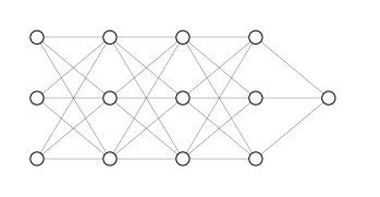
When applying regularization we will add the term $\frac{\lambda}{2m} \sum_{l=1}^L |w^{[l]}|^2$ to the cost function $J(w^{[l]}, b^{[l]})$. In this way we will increase the cost for high values of $w^{[l]}$ and bring gradient descent to reduce the values $w^{[l]}$.
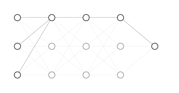
For a sufficiently high value of the regularization parameter $\lambda$, we will have $w^{[l]} \approx 0$. In turn, this will give $a^{[l]} \approx 0$ for some nodes (Figure 49), reducing the complexity of the functions encoded by the neural network.
Forcing hidden units to linearity
A second way to imagine the effect of regularization on gradient descent is that if thinking that, by reducing the values of the parameters $w$, regularized gradient descent forces the activation values $a$ to be linear.
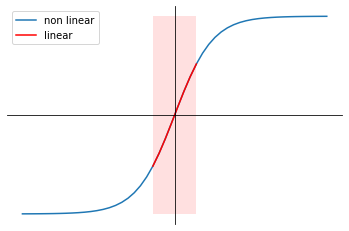
Suppose you have an hidden unit with activation function $g(z) = \tanh(z)$. Having a sufficiently high regularization parameter $\lambda$ implies that the values of the parameter matrix $w^{[l]}$ will deviate from extreme values and tend to 0.
When the activation function (tanh in this case) is applied to $z$, since the latter falls in values close to 0, $g(z)$ will be mostly linear (figure below). A combination of any number of linear hidden units will result in a linear model.