Dropout

A very powerful regularization technique is called dropout.

In dropout we will assign for each layer a probability $p$ of retaining each node in the layer (Figure 51). We will then randomly remove a different set of nodes for each examples, according to their layer probabilities. So for each training example you will train the model using a random reduced network.

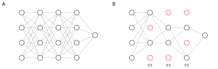
The effect of dropout is to spread the weights across hidden units during training. Since sometimes some of the hidden units are unavailable, the model is trained not to “rely” on any single unit. The spreading of weights has a similar effect as $L_2$ regularization and, while they have some different implications, they tend to have a pretty similar effect.

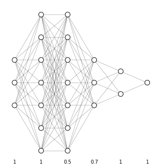
The retain probability $p$ can be set at a different value for each layer and usually is set lower for layer that have more risk to suffer from overfitting. For example, suppose we have the neural network represented in Figure 52: we would retain all nodes in the input layer ($p=1$) and and the first layer ($w \in \mathbb{R}^{7, 1}$); apply a rather low retain probability to the second layer ($w \in \mathbb{R}^{7, 7}$), which is the layer that has the most probability to suffer from overfitting, an higher retain probability to the third layer ($w \in \mathbb{R}^{3, 7}$) and keep all other units.

One downside of dropout is to render the cost function $J$ undefined: this means that training surveillance methods such as plotting the value of $J$ at each iteration (to ensure that it is decreasing) are no longer valid.

Implementing dropout (inverted dropout)

Let’s suppose to implement dropout for layer $l=3$. We will define a vector of dropout probabilities $d^{[3]}$ based on the keep probability $p = 0.8$ that represents the probability that each hidden unit is not discarded.

# a3 = forward_prop()
p = 0.8 # keep probability
d3 = np.random.rand(*a3.shape) < p
a3 *= d3
a3 /= p # inverted dropout

The last operation is used to counterbalance the random elimination of hidden units. In fact, continuing in forward propagation we would have:

So by applying $a^{[3]} = \frac{a^{[3]}}{0.8}$ we would bump up the values of $a^{[3]}$ by 20% and counter the reduction produced shutting nodes off. This is called the inverted dropout technique and ensures that, independently from the value of $p$, the expected value of $a$ remains the same.

Inverted dropout removes the need to scale up parameters at test time. In fact, at test time you will just forward propagate from input to prediction and, by applying the inverted dropout the activation scale is automatically correct.

Other regularization methods

Data augmentation

When you have a large number of input features, as in the case of image recognition, you will probably never have enough training data and your model is almost guaranteed to overfit. Since the option of getting more data (which would be the best option) is ruled out a priori, you can try and get around this problem by artificially producing more data, an approach called data augmentation.

The principle of data augmentation is to apply some transform function to the data you have in order to produce a slightly different form of your data that will help to build a more robust (generalized) model.

For example if you are training an image recognition algorithm, you could flip all images horizontally, rotate and skew the image, add some blur, … .

Early stopping

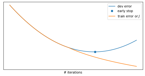
When training your neural network, you can plot the training and dev set error as a function of the number of iterations to diagnose over- or under-fitting problems. The plots will usually look like that in Figure 53, where the train error will decrease monotonically while the number of iterations increase and the dev set error will decrease up to a certain point where it starts to rise back up. This is due to the fact that after the flex point we are overfitting our model to the training data and this loss of generalization decrease its performance on the dev set.

In early stopping you stop the training when the dev set error flexes back up. The principle behind this is that at the very start of the model training the parameters will be very small ($w \approx 0$ due to random initialization) and they will gradually increase and become bigger and bigger while iterating. With early stopping we obtain mid-size parameters, an effect very similar to $L_2$ regularization ($| w |_F^2$)

Early stopping has the disadvantage to inextricably coupling two processes:

• optimize the cost function $J$: reach the minimum of the cost function by tuning the hyperparameters and bringing gradient descent to convergence
• reduce overfitting (variance): apply regularization. Once the optimization step is complete you will most likely have an overfitted model, in this step you reduce the overfitting to try to generalize your model.

Keeping this two step separated is called orthogonalization and is a recommended approach in most cases, but with early stopping you couple this two tasks and try to both optimize $J$ and prevent overfitting in one go.

On the other hand, by using $L_2$ regularization you need to try many values of the hyperparameter $\lambda$ and this may become computationally heavy, while with early stopping you train and regularize in one go and it’s much more computationally efficient.

Comments